Phyllochron

Phyllochron is a model that estimates how quickly new leaves appear on a wheat plant after it emerges from the soil. This timing is important because it influences later growth stages and ultimately affects crop yield and development.

Overview

The Phyllochron model simulates the interval between the appearance of successive leaf tips on a wheat plant. It acts like a biological clock, helping researchers and agronomists predict how fast a plant will grow new leaves under different conditions. This model is a key part of the crop’s phenology (developmental timing), which is crucial for understanding when the plant will reach important stages like flowering and grain filling.

Leaf appearance rate is influenced by temperature (how warm it is), the plant’s stage of development (which leaf is appearing), and the length of the day (photoperiod). By adjusting these parameters, the model can represent different wheat varieties and growing environments. This helps breeders and agronomists select varieties that are better suited to specific climates or management practices.

Methodology

The Phyllochron model is based on the idea that the time between new leaf appearances (measured in degree-days, or °C·days) is not constant. Instead, it changes depending on the leaf’s position on the plant and the day length.

The effective phyllochron (\(P_{\text{eff}}\)) is calculated as:

\[ P_{\text{eff}} = P_{\text{base}} \times f_{\text{leaf}}(n) \times f_{\text{pp}}(d) \]

\(P_{\text{base}}\) is the base phyllochron (default: 120 °C·days), representing the typical interval between leaves under standard conditions for leaf rank from 3 to 7.
\(f_{\text{leaf}}(n)\) is a factor that adjusts the phyllochron depending on which leaf is appearing (\(n\) is the leaf cohort number).
\(f_{\text{pp}}(d)\) is a modifier that accounts for the effect of day length (\(d\) is the photoperiod in hours).

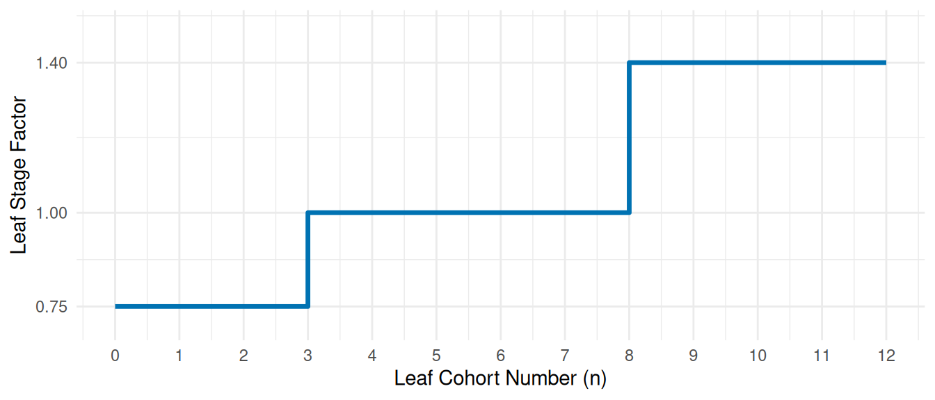
Leaf Stage Factor

The rate at which new leaves appear changes as the plant grows. Early leaves appear faster, while later leaves take longer (Jamieson et al. 1998). This is represented by a piecewise function:

Leaf Cohort Number (\(n\))	Factor
0–2	0.75
3–7	1.0
8+	1.4

This means the first 2 leaves appear more quickly, leaves in the middle appear at a standard rate, and later leaves appear more slowly.

Leaf Stage Factor as a Function of Leaf Cohort Number

Photoperiod Effect

The model also accounts for how sensitive the plant is to day length with 6 degrees twilight. When days are short (less than 12 hours), leaf appearance slows down. The photoperiod effect is calculated as:

\[ f_{\text{pp}}(d) = 1 + S \cdot f_d(d) \]

\(S\) is the photoperiod sensitivity (a parameter that can be adjusted for different varieties). \(S\) is typically set to 0.6 for wheat, which means the phyllochron increases by 60% (i.e. \(120 \times (1 + 0.6) = 192\) °C·days) when day length is less than 8 hours, and not at all (i.e. \(120 \times (1 + 0) = 120\) °C·days) when it is above 12 hours.
\(f_d(d)\) describes how the effect changes with day length:

Day Length (h)	Modifier \(f_d(d)\)
8	1.0
12	0.0
20	0.0

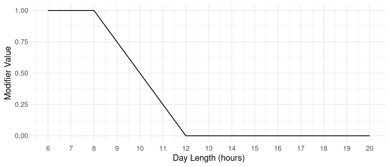
So, for day lengths below 12 hours, the phyllochron increases (leaves appear more slowly), but above 12 hours, there is no further effect.

Cultivar-Specific Parameters

Name	Description	Default Value
[Phenology].PhyllochronPpSensitivity.FixedValue	Sensitivity of leaf appearance rate to photoperiod	0.6
[Phenology].Phyllochron.BasePhyllochron.FixedValue	Base phyllochron	120

Practical Example

Leaf Rank Effects

We assume a wheat cultivar with a base phyllochron of 100 °C·days, a photoperiod sensitivity of 0.6, and sown at Inverleigh, Victoria, which has a day length of 11 hours in winter. The phyllochron for leaf 1 to 8 can be calculated as follows:

Base phyllochron (\(P_{\text{base}}\)): 100 °C·days
Photoperiod modifier (\(f_{\text{pp}}(11)\)):
- \(f_d(11) = \frac{12 - 11}{12 - 8} = 0.25\)
- \(f_{\text{pp}}(11) = 1 + 0.6 \times 0.25 = 1.15\)
Leaf stage factor (\(f_{\text{leaf}}(n)\)):
- Leaves 1–2: 0.75
- Leaves 3–7: 1.0
- Leaf 8: 1.4

Example calculations:

This table shows the phyllochron for each leaf cohort under these example conditions.

Leaf Cohort (\(n\))	\(f_{\text{leaf}}(n)\)	\(P_{\text{eff}}\) (°C·days)
1	0.75	\(100 \times 0.75 \times 1.15 = 86.25\)
2	0.75	\(100 \times 0.75 \times 1.15 = 86.25\)
3	1.0	\(100 \times 1.0 \times 1.15 = 115.0\)
4	1.0	\(100 \times 1.0 \times 1.15 = 115.0\)
5	1.0	\(100 \times 1.0 \times 1.15 = 115.0\)
6	1.0	\(100 \times 1.0 \times 1.15 = 115.0\)
7	1.0	\(100 \times 1.0 \times 1.15 = 115.0\)
8	1.4	\(100 \times 1.4 \times 1.15 = 161.0\)

Effect of Photoperiod Sensitivity

To illustrate how photoperiod sensitivity (\(S\)) affects the phyllochron, let’s calculate \(P_{\text{eff}}\) for a range of \(S\) values from 0 to 1 (at 0.2 intervals) with a fixed day length of 10 hours. We’ll use a base phyllochron of 100 °C·days and the leaf stage factor for leaf 3 (\(f_{\text{leaf}}(3) = 1.0\)).

First, calculate \(f_d(10)\): - \(f_d(10) = \frac{12 - 10}{12 - 8} = \frac{2}{4} = 0.5\)

Now, for each \(S\):

Photoperiod Sensitivity (\(S\))	\(f_{\text{pp}}(10)\)	\(P_{\text{eff}}\) (°C·days)
0.0	\(1 + 0.0 \times 0.5 = 1.00\)	\(100 \times 1.0 \times 1.00 = 100.0\)
0.2	\(1 + 0.2 \times 0.5 = 1.10\)	\(100 \times 1.0 \times 1.10 = 110.0\)
0.4	\(1 + 0.4 \times 0.5 = 1.20\)	\(100 \times 1.0 \times 1.20 = 120.0\)
0.6	\(1 + 0.6 \times 0.5 = 1.30\)	\(100 \times 1.0 \times 1.30 = 130.0\)
0.8	\(1 + 0.8 \times 0.5 = 1.40\)	\(100 \times 1.0 \times 1.40 = 140.0\)
1.0	\(1 + 1.0 \times 0.5 = 1.50\)	\(100 \times 1.0 \times 1.50 = 150.0\)

References

Jamieson, P. D., M. A. Semenov, I. R. Brooking, and G. S. Francis. 1998. “Sirius: A Mechanistic Model of Wheat Response to Environmental Variation.” European Journal of Agronomy 8 (3–4): 161–79. https://doi.org/16/S1161-0301(98)00020-3.