XYPairs

Returns the corresponding Y value for a given X value, based on the line shape defined by the specified XY matrix.

Overview

XYPairs is a fundamental function in APSIM NG that defines response curves by specifying a series of X and Y coordinate pairs. For a given input X value, it returns a linearly interpolated Y value based on the defined XY matrix. If the input X value falls outside the defined range, the function returns the Y value at the nearest boundary point (either the first or last Y value).

This function is particularly useful for modeling empirical relationships where measured data is available, such as temperature response curves, biomass partitioning coefficients, or developmental rate functions in agricultural models. It provides a flexible way to represent non-linear relationships without requiring specific mathematical formulations.

Model Structure

This section describes how this model is positioned within the APSIM framework. It outlines the broader structural and computational components that define its role and interactions in the simulation system.

This model inherits structural and functional behaviour from the following core APSIM components:

Connections to Other Components

This section describes how the model interacts with other components in the APSIM Next Generation framework.
These connections allow the model to exchange information—such as environmental conditions, developmental stage, or physiological responses—with other parts of the simulation system. For a general overview of how model components are connected in APSIM, see the Connections Overview.

XYPairs is typically used as a child function within other model components. It does not directly link to other models but receives its input X value from the parent model that calls it. The function can be used anywhere an IFunction or IIndexedFunction interface is expected.

Model Variables

This section lists the key variables that describe or control the behaviour of this component. Some variables can be adjusted by the user to modify how the model behaves (configurable), while others are calculated internally and can be viewed as model outputs (reportable). For a general explanation of variable types and how they are used within the APSIM Next Generation framework, see the Model Variables Overview.

Configurable and Reportable Properties

Property	Type	Description
X	double[]	Array of X values defining the input domain. These values should be in ascending order.
Y	double[]	Array of Y values corresponding to each X value. Must be the same length as X.

Read-Only Reportable Properties

No read-only properties are available for this function.

Processes and Algorithms

This section describes the scientific processes and algorithms represented by this component. Each process corresponds to a biological, physical, or chemical mechanism simulated during a model time step. Where appropriate, equations or conceptual summaries are provided to explain how the process operates within the APSIM Next Generation framework.

Linear Interpolation

The XYPairs function performs linear interpolation between user-defined X and Y value pairs. When the function is called with an input X value (\(dX\)), it locates the segment of the curve that contains the input and linearly interpolates to determine the corresponding Y value.

The interpolation follows this equation between two consecutive points \((x_i, y_i)\) and \((x_{i+1}, y_{i+1})\):

\[ Y = y_i + \frac{(dX - x_i)}{(x_{i+1} - x_i)} (y_{i+1} - y_i) \]

where: - \(dX\) is the input X value - \(x_i\) and \(x_{i+1}\) are the two consecutive X values in the array that bracket \(dX\) - \(y_i\) and \(y_{i+1}\) are the corresponding Y values

Boundary Behavior

If the input X value falls outside the defined X range: - For \(dX < x_1\) (below the minimum), the function returns \(y_1\) (the first Y value) - For \(dX > x_n\) (above the maximum), the function returns \(y_n\) (the last Y value)

This behavior ensures the function always returns a valid value and is particularly useful for extrapolation scenarios where the model operates at the limits of the defined response curve.

User Interface

XYPairs can be added as a child of any model that requires a function in the model tree. Right-click the parent node, select “Add Model…”, and search for XYPairs in the Filter Box.

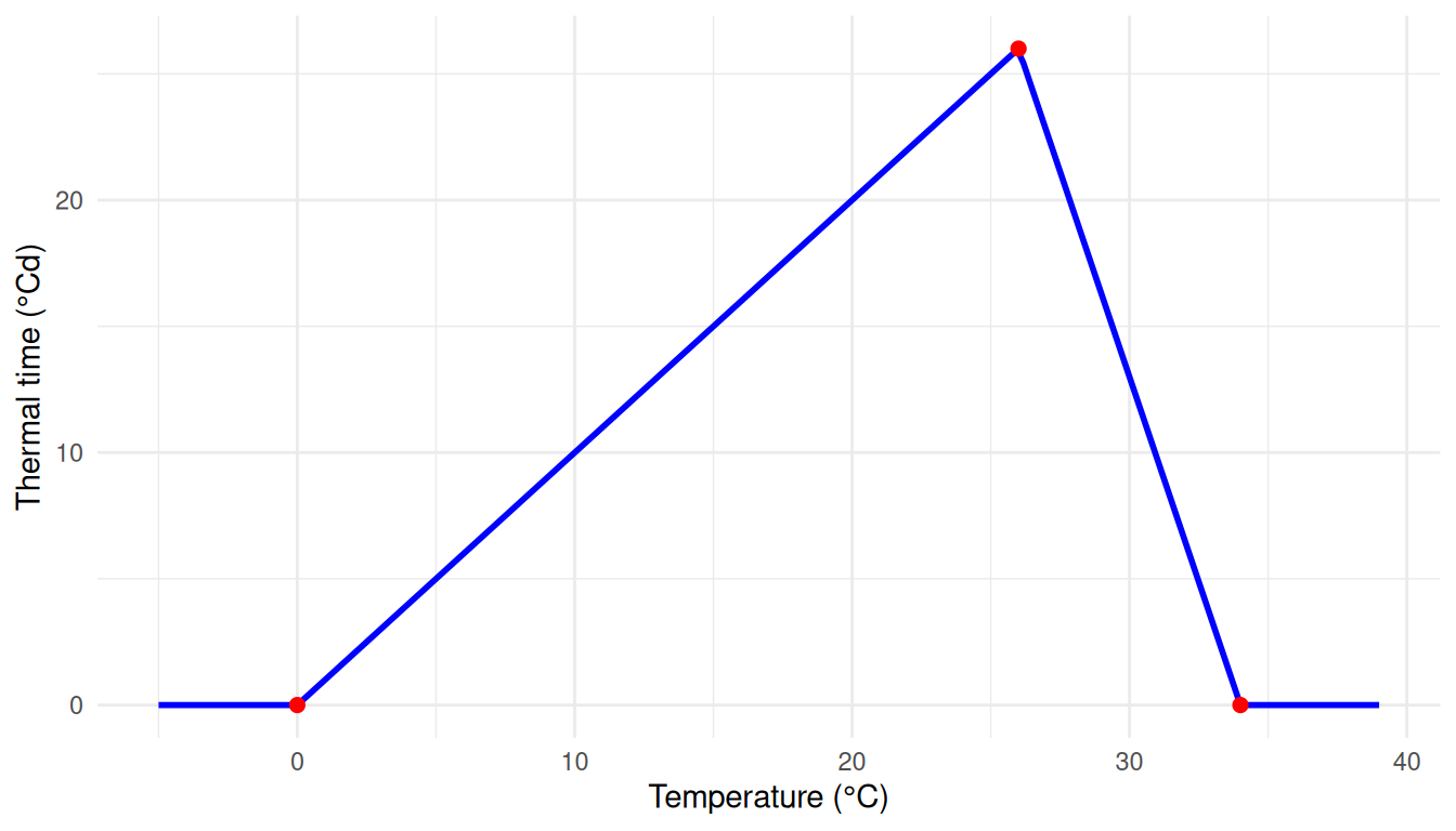
Practical Example

Suppose you want to define a thermal time response curve for a developmental process that increases linearly with temperature up to an optimal value, then decreases. This might represent enzyme activity or photosynthetic rate as a function of temperature.

Set:

X = [0, 26, 34] (Temperature in °C)
Y = [0, 26, 0] (Thermal time accumulation in °Cd)

This configuration means: - For temperatures below 0°C, thermal time accumulation is 0 (development ceases) - From 0 to 26°C, thermal time increases linearly from 0 to 26°Cd per day - From 26 to 34°C, thermal time decreases linearly from 26 to 0°Cd per day - For temperatures above 34°C, thermal time accumulation is 0 (heat stress stops development)

Example of XYPairs function showing thermal time accumulation as a function of temperature